NJOAG Use of Force and Law Enforcement Officer Diversity data sets
The NJ Office of the Attorney General has started releasing data on police use of force and on law enforcement officer diversity, which I have re-packaged as R data packages NJOAGUOF and NJOAGLEOD.
I’d like to start digging into this data to see what it shows. I’ll start with the municipal agencies – in particular, agency sizes. 1
Packages used in this post
In this post, I’ll be using the following packages.| Package | Title | Version |
|---|---|---|
| njoagleod | NJ OAG Law Enforcement Officer Diversity data package | 1.1.3 |
| tidyverse | Easily Install and Load the ‘Tidyverse’ | 1.3.1 |
| tidycensus | Load US Census Boundary and Attribute Data as ‘tidyverse’ and ‘sf’-Ready Data Frames | 1.2.2 |
| tigris | Load Census TIGER/Line Shapefiles | 1.6.1 |
| sf | Simple Features for R | 1.0-7 |
| ggrepel | Automatically Position Non-Overlapping Text Labels with ‘ggplot2’ | 0.9.1 |
This is not a tutorial for using these packages, but all the R code used to generate the plots and tables will be included.
Both NJOAG packages mentioned above may be installed from github, though we will only use njoagleod in this post.
install_github("tor-gu/njoaguof")
install_github("tor-gu/njoagleod")
Municipal agencies and census data
Building a population and officer_count table by municipality
Let’s start by getting municipal-level census data using the tidycensus package. 2 We will use the municipality table in the njoagleod package for the list of counties. For the moment, we only need the population of each municipality.
library(tidyverse)
library(tidycensus)
library(njoagleod)
# Get a vector of NJ counties
counties <- municipality %>% pull(county) %>% unique() %>% sort()
# Get the population of each municipality using tidycensus::get_estimates
municipality_pop <- counties %>%
  map_df(
    ~ get_estimates(
      geography = "county subdivision",
      state = "NJ",
      county = .,
      year = 2019,
      variables = "POP"
    ) %>%
      separate(
        NAME,
        sep = ", ",
        into = c("municipality", "county", "state")
      )
  ) %>%
  rename(population=value) %>%
select(-variable, -state)| municipality | county | GEOID | population |
|---|---|---|---|
| Buena borough | Atlantic County | 3400108680 | 4284 |
| Egg Harbor City city | Atlantic County | 3400120350 | 4052 |
| Hamilton township | Atlantic County | 3400129280 | 25746 |
| Mullica township | Atlantic County | 3400149410 | 5856 |
| Somers Point city | Atlantic County | 3400168430 | 10174 |
| Absecon city | Atlantic County | 3400100100 | 8818 |
Now let’s get the officer count for each municipal police department and combine it with the census data. Not every municipality has its own police department, and there may be municipal police departments that are excluded for some reason (for example, because they have not reported their data to the OAG).
# Get the officer count for each agency
officer_count_pop <- officer %>%
  count(agency_county, agency_name, name = "officer_count") %>%
  left_join(agency,
            by = c("agency_county", "agency_name")) %>%
  filter(!is.na(municipality)) %>%
  left_join(municipality,
            by = c("agency_county" = "county", "municipality")) %>%
  select(GEOID, agency_name, officer_count) %>%
left_join(municipality_pop, by = "GEOID")| GEOID | agency_name | officer_count | municipality | county | population |
|---|---|---|---|---|---|
| 3400100100 | Absecon City PD | 29 | Absecon city | Atlantic County | 8818 |
| 3400102080 | Atlantic City PD | 257 | Atlantic City city | Atlantic County | 37743 |
| 3400107810 | Brigantine PD | 35 | Brigantine city | Atlantic County | 8650 |
| 3400120350 | Egg Harbor City PD | 17 | Egg Harbor City city | Atlantic County | 4052 |
| 3400120290 | Egg Harbor Twp PD | 92 | Egg Harbor township | Atlantic County | 42249 |
| 3400125560 | Galloway Twp PD | 70 | Galloway township | Atlantic County | 35618 |
Checking that the table is representative of New Jersey.
As we mentioned above, our officer_count_pop table will not include a row for every municipality of NJ. Before digging in too far, let’s get a sense of what we are including and what we are missing.
Statewide, the municipal agencies for which we have data cover nearly 93% of the population of New Jersey. In all, there are about 408 residents per municipal police officer in these municipalities.
# We cover nearly 93% of the population of NJ
sum(officer_count_pop$population) / sum(municipality_pop$population)
## [1] 0.93# About 408 residents per municipal police officer
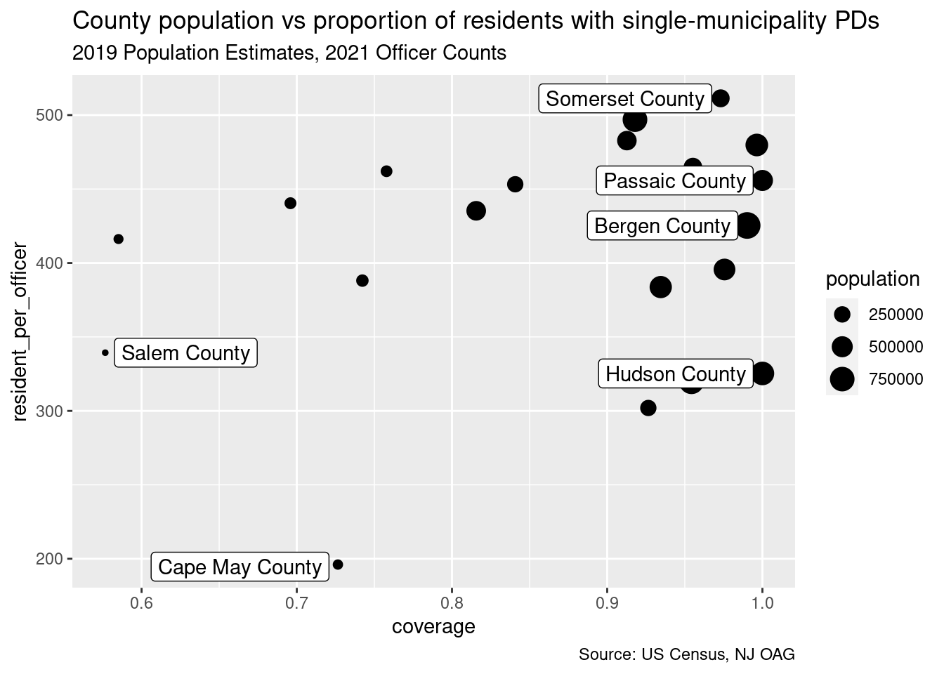
sum(officer_count_pop$population) / sum(officer_count_pop$officer_count)## [1] 408At the county level, the coverage varies from from about 58% of the population (Salem county) up to 100% (Hudson and Passaic), and the number of residents per officer ranges from 511 (Somerset) to 196 (Cape May). Note that in Cape May, our data covers only 73% of the population.
# Get the population for each municipality that is 'missed' and summarize by
# county
missed_county_pop <- municipality_pop %>%
  anti_join(officer_count_pop, by = "GEOID") %>%
  group_by(county) %>%
  summarize(missed_population = sum(population))
# Get the total population by county
county_pop <- municipality_pop %>%
  group_by(county) %>%
  summarize(population = sum(population))
# Combine this to get the county-level coverage -- the proportion of the
# population of each county with a municipal PD for which we have the data
coverage <- county_pop %>%
  left_join(missed_county_pop, by = "county") %>%
  mutate(missed_population = replace_na(missed_population, 0)) %>%
  mutate(coverage = (population - missed_population) / population) %>%
  select(county, missed_population, coverage)
# Now add the county-level municipal PD officer count
officer_count_pop_by_county <- officer_count_pop %>%
  group_by(county) %>%
  summarize(officer_count = sum(officer_count),
            population = sum(population)) %>%
  mutate(resident_per_officer = population / officer_count) %>%
left_join(coverage, by = "county")| county | officer_count | population | resident_per_officer | missed_population | coverage |
|---|---|---|---|---|---|
| Atlantic County | 809 | 244289 | 302 | 19381 | 0.93 |
| Bergen County | 2170 | 923035 | 425 | 9167 | 0.99 |
| Burlington County | 842 | 406464 | 483 | 38885 | 0.91 |
| Camden County | 949 | 413077 | 435 | 93394 | 0.82 |
| Cape May County | 341 | 66866 | 196 | 25173 | 0.73 |
| Cumberland County | 286 | 110990 | 388 | 38537 | 0.74 |
| Essex County | 2385 | 762478 | 320 | 36497 | 0.95 |
| Gloucester County | 541 | 245192 | 453 | 46444 | 0.84 |
| Hudson County | 2067 | 672391 | 325 | 0 | 1.00 |
| Hunterdon County | 204 | 94252 | 462 | 30119 | 0.76 |
| Mercer County | 755 | 350981 | 465 | 16449 | 0.96 |
| Middlesex County | 1524 | 757317 | 497 | 67745 | 0.92 |
| Monmouth County | 1507 | 578260 | 384 | 40535 | 0.93 |
| Morris County | 983 | 448845 | 457 | 43000 | 0.91 |
| Ocean County | 1261 | 604996 | 480 | 2190 | 1.00 |
| Passaic County | 1101 | 501826 | 456 | 0 | 1.00 |
| Salem County | 106 | 35971 | 339 | 26414 | 0.58 |
| Somerset County | 626 | 320092 | 511 | 8842 | 0.97 |
| Sussex County | 222 | 97770 | 440 | 42718 | 0.70 |
| Union County | 1372 | 542753 | 396 | 13588 | 0.98 |
| Warren County | 148 | 61596 | 416 | 43671 | 0.59 |
Though the outliers like Cape May and Hudson may suggest a correlation between our coverage rate and the number of residents per officer – which would in turn suggest we may be oversampling municipalities with larger police departments – the actual correlation is not significant:
# Weighted by population, there is no significant correlation between
# residents_per_officer and our coverage.
lm(resident_per_officer ~ coverage,
   officer_count_pop_by_county,
   weights = population) %>%
  summary() %>%
  magrittr::use_series("coefficients")
## Estimate Std. Error t value Pr(>|t|)
## (Intercept) 430 184 2.334 0.031
## coverage -11 196 -0.054 0.957# Plot number of residents per officer by coverage
outliers <- officer_count_pop_by_county %>%
filter(
population == min(population) | population == max(population) |
coverage == min(coverage) | coverage == max(coverage) |
resident_per_officer == min(resident_per_officer) |
resident_per_officer == max(resident_per_officer)
)
officer_count_pop_by_county %>%
ggplot(aes(x = coverage, y = resident_per_officer)) +
geom_point(aes(size = population)) +
ggrepel::geom_label_repel(data = outliers, aes(label = county)) +
labs(
title =
str_wrap(
"County population vs proportion of residents with single-municipality PDs"
),
subtitle = "2019 Population Estimates, 2021 Officer Counts",
caption = "Source: US Census, NJ OAG"
)
Mapping municipalities with large police departments relative to their population
Now that we have our data set, let’s take a look at the municipalities with the largest police departments relative to their population:
top_fifteen <- officer_count_pop %>%
  mutate(residents_per_officer = population / officer_count) %>%
  slice_min(n = 15, order_by = residents_per_officer) %>%
  select(agency_name,
         county,
         residents_per_officer,
         officer_count,
population)| agency_name | county | residents_per_officer | officer_count | population |
|---|---|---|---|---|
| Mantoloking Boro PD | Ocean County | 28 | 9 | 249 |
| Deal PD | Monmouth County | 34 | 21 | 719 |
| Harvey Cedars Boro PD | Ocean County | 38 | 9 | 345 |
| Stone Harbor Boro PD | Cape May County | 48 | 17 | 810 |
| Allenhurst PD | Monmouth County | 54 | 9 | 483 |
| Avalon Boro PD | Cape May County | 56 | 22 | 1236 |
| Longport PD | Atlantic County | 61 | 14 | 851 |
| Hi-Nella PD | Camden County | 78 | 11 | 858 |
| Sea Isle City PD | Cape May County | 85 | 24 | 2029 |
| Lavallette PD | Ocean County | 85 | 22 | 1866 |
| Long Beach Twp PD | Ocean County | 88 | 35 | 3071 |
| Ship Bottom Boro PD | Ocean County | 89 | 13 | 1153 |
| Beach Haven PD | Ocean County | 93 | 13 | 1205 |
| Bayhead Boro PD | Ocean County | 109 | 9 | 977 |
| Surf City PD | Ocean County | 109 | 11 | 1199 |
In case the names of these relatively smaller municipalities don’t mean much to you, let’s take a look at them on a map. We’ll use the tigris package to get the shapefiles for the municipalities from the US census:
library(tigris)
options(tigris_use_cache = TRUE)
nj_municipality_map <- counties %>%
  map_df( ~ county_subdivisions("NJ", county = ., class = "sf"))
Next we join the officer count data to the map and plot.
# Add the residents_per_officer to the map
officer_count_pop <- officer_count_pop %>%
  mutate(residents_per_officer = population / officer_count)
map_with_values <-
  left_join(nj_municipality_map, officer_count_pop, by = "GEOID")

# Select the top values for labeling
labels <- map_with_values %>%
  slice_min(n = 15, order_by = residents_per_officer) %>%
  arrange(desc(INTPTLAT))

# Map the officer density
scale_breaks <- c(30, 40, 60, 120)
ggplot(map_with_values) +
  geom_sf(aes(fill = residents_per_officer, geometry = geometry, size = .2 )) +
  ggrepel::geom_label_repel(
    data = labels,
    mapping = aes(label = NAME, geometry = geometry),
    stat = "sf_coordinates",
    nudge_x = -.7,
    min.segment.length = 0
  ) +
  scale_size_identity() +
  scale_fill_gradient(
    na.value = "lightgrey",
    low = "white",
    high = "red",
    trans = "reciprocal",
    breaks = scale_breaks,
    name = "Residents Per Officer"
  ) +
  labs(
    title = str_wrap(
      "NJ municipalities with large police departments relative to population"
    ),
    subtitle = "2019 Population Estimates, 2021 Officer Counts",
    caption = "Source: US Census, NJ OAG"
  ) +
  theme(
    axis.ticks = element_blank(),
    axis.text.x = element_blank(),
    axis.text.y = element_blank(),
    axis.title.x = element_blank(),
    axis.title.y = element_blank(),
    panel.background = element_rect(fill = "lightblue"),
    panel.grid.major = element_line(color = "lightblue"),
    legend.position = "bottom"
  )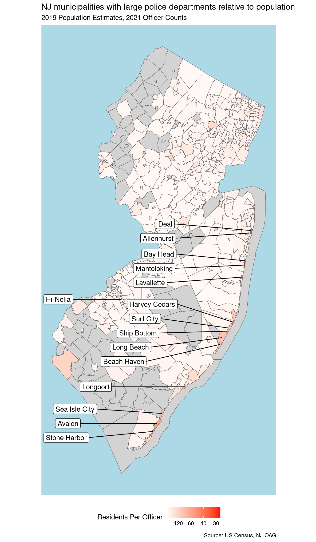
So, a map of the largest percapita municipal PDs in NJ is a map of the Jersey Shore, plus Hi-Nella.
Part-time residents and part-time officers
Hi-Nella
Before we get to the shore towns, let’s take a quick look at the borough of Hi-Nella. A population of 858 and 11 police officers – that sure seems like a lot!
Back in 2010, the Star-Ledger reported on Hi-Nella (Towns that Shouldn’t Exist Part 2: Borough of Hi-Nella). At that time, the population was 1029 and the police department had 13 officers. But, the Star-Ledger notes, this a “mostly part-time police force”.
The NJ OAG data set does not distinguish part-time from full-time officers, so it is not clear how much of the Hi-Nella PD is part time. The Hi-Nella PD website lists a Chief, a Lieutenant and a Detective, presumably all full-time, and no other officers. Perhaps the department has three full-time and 8 part-time officers, which is still on the large side.
Jersey Shore towns
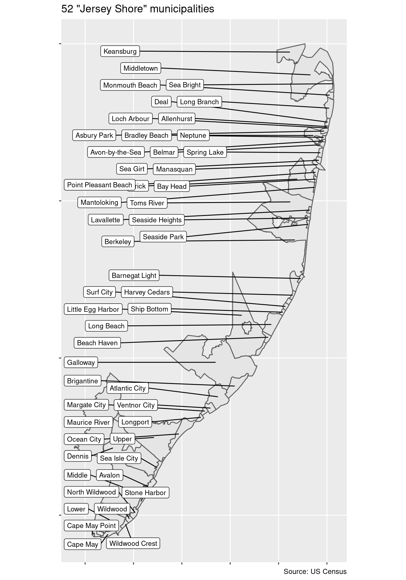
The other fourteen agencies on the list are all on the Jersey Shore. The most extreme example is Mantoloking, with 9 officers and only 249 residents.
Mantoloking
The wikipedia page for Mantoloking gives a good explanation for why this might be: during the summer months, the population swells to approximately 5000. For a populuation of 5000, nine officers is actually lower than the state average: more than 500 residents per officer. Indeed, the Mantoloking PD website indicates that the department hires seasonal officers in the summer, and that it has nine full-time officers.
Note the contrast with Hi-Nella – both Hi-Nella and Mantoloking employ part-time officers, but part-time officers in Hi-Nella are included in the agency size, while part-time officers in Mantoloking are excluded. It is not clear how most departments have counted their part-time officers. 3
Returning the the shore towns, it is clear that many of them have seasonal patterns similar to Mantoloking. For example, Deal’s population increases ten-fold in the summer.
Isolating the shore towns
The NJ map includes several landless non-municipal county subdivisions off the coast, which we can identify by filtering on ALAND == 0.
# Select the landless regions and plot the GEOIDs
water <- nj_municipality_map %>% filter(ALAND == 0)
ggplot(nj_municipality_map) +
  geom_sf(aes(geometry = geometry)) +
  geom_sf_label(data = water,
                mapping = aes(label = GEOID, geometry = geometry)) +
  labs(title = str_wrap("Landless county subdivision GEOIDs in NJ"),
       caption = "Source: US Census") +
  theme(
    axis.text.x = element_blank(),
    axis.text.y = element_blank(),
    axis.title.x = element_blank(),
    axis.title.y = element_blank()
  )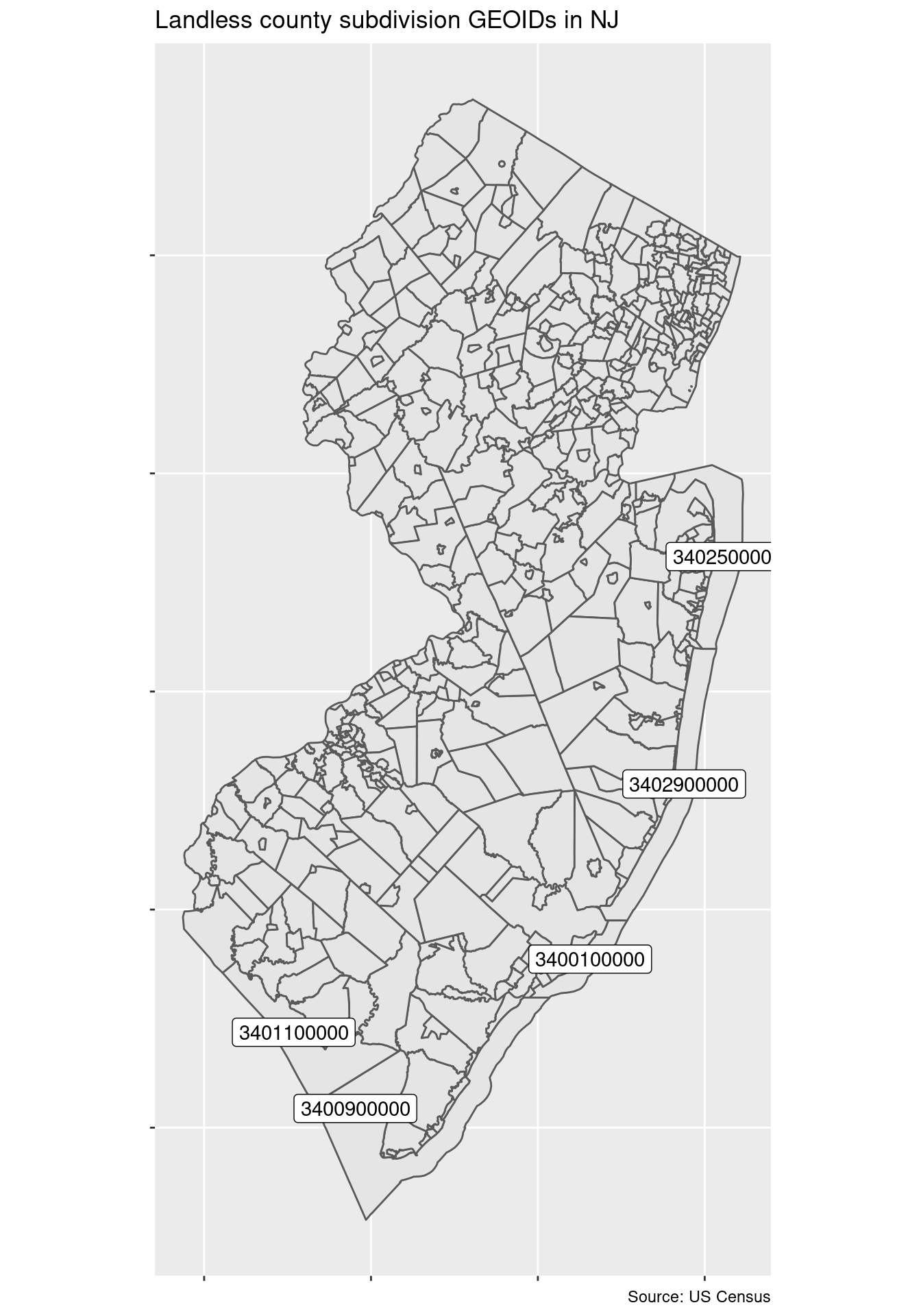
We can take a stab at defining the “Jersey Shore” as those municipalities that border any of these regions, excluding the Delaware Bay region 3401100000.
# Build the jersey shore map
jersey_shore_water <- water %>% filter(GEOID != "3401100000")
jersey_shore_indices <-
sf::st_intersects(jersey_shore_water, nj_municipality_map) %>%
unlist() %>% unique()
jersey_shore <-
nj_municipality_map[jersey_shore_indices, ] %>% setdiff(water)
# Plot the jersey_shore towns
ggplot(jersey_shore) + geom_sf() +
ggrepel::geom_label_repel(
mapping = aes(label = NAME, geometry = geometry),
stat = "sf_coordinates",
nudge_x = -.7,
min.segment.length = 0,
size = 3
) +
labs(title = str_wrap("52 \"Jersey Shore\" municipalities"),
caption = "Source: US Census") +
theme(
axis.text.x = element_blank(),
axis.text.y = element_blank(),
axis.title.x = element_blank(),
axis.title.y = element_blank()
) Now we can add a flag,
 shore_town, to the officer_count_pop table:
officer_count_pop <- officer_count_pop %>%
mutate(shore_town=GEOID %in% jersey_shore$GEOID)| GEOID | agency_name | officer_count | municipality | county | population | residents_per_officer | shore_town |
|---|---|---|---|---|---|---|---|
| 3400100100 | Absecon City PD | 29 | Absecon city | Atlantic County | 8818 | 304 | FALSE |
| 3400102080 | Atlantic City PD | 257 | Atlantic City city | Atlantic County | 37743 | 147 | TRUE |
| 3400107810 | Brigantine PD | 35 | Brigantine city | Atlantic County | 8650 | 247 | TRUE |
| 3400120350 | Egg Harbor City PD | 17 | Egg Harbor City city | Atlantic County | 4052 | 238 | FALSE |
| 3400120290 | Egg Harbor Twp PD | 92 | Egg Harbor township | Atlantic County | 42249 | 459 | FALSE |
| 3400125560 | Galloway Twp PD | 70 | Galloway township | Atlantic County | 35618 | 509 | TRUE |
Comparing the Jersey Shore to the rest of the state
As expected, the small Jersey Shore towns (like Mantoloking and Deal) have noticeably larger police forces relative to their population than the rest of the state. But this distinction starts to break down with larger shore towns:
# Plot the officer count vs the population for small and medium towns,
# separating the shore towns from the rest of the state
officer_count_pop %>%
  mutate(town_size = factor(
    case_when(
      population < 5000 ~ "Small",
      population < 50000 ~ "Medium",
      TRUE ~ "Large"
    ),
    levels = c("Small", "Medium", "Large")
  )) %>%
  filter(town_size != "Large") %>%
  ggplot(aes(x = population, y = officer_count, color = shore_town)) +
  geom_point() +
  geom_smooth(se = FALSE, method="loess") +
  facet_wrap("town_size", scales = "free") +
  labs(title = "NJ Residents Per Municipal Law Enforcement Officer",
       subtitle = "Small and Medium Sized Towns, Jersey Shore vs Rest of State",
       caption = "Source: US Census, NJ OAG") +
  theme(legend.position = "bottom")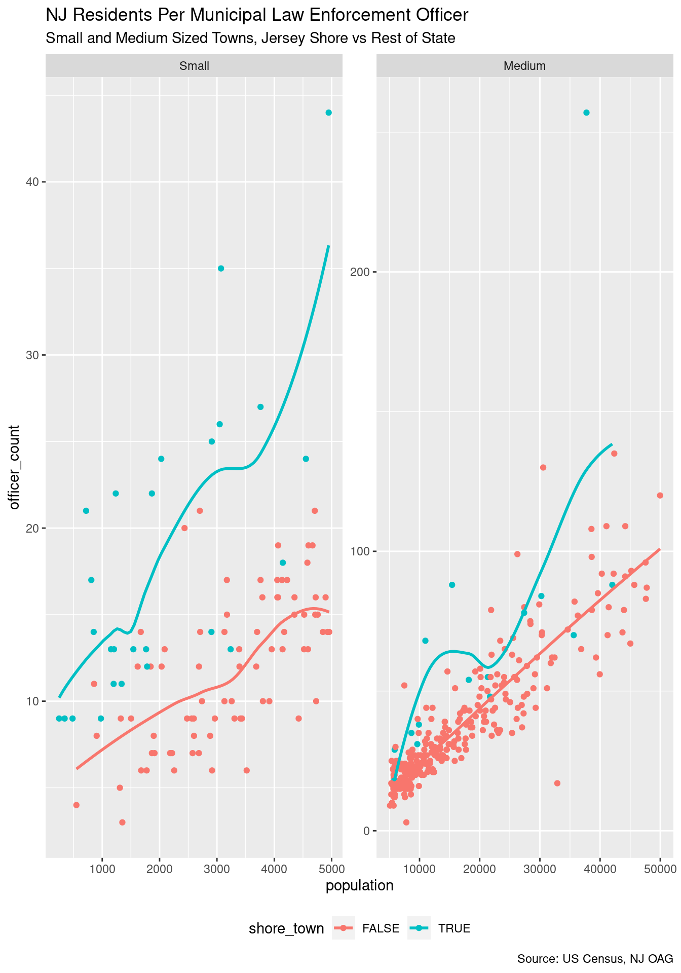
If we look at just the 26 small shore towns – population at most 5000 – the number of residents per officer is 111, compared to 415 for the rest of the state:
shore_vs_non_shore <- officer_count_pop %>%
  mutate(small_shore_town = (population <= 5000 & shore_town)) %>%
  group_by(small_shore_town) %>%
  summarise(officer_count = sum(officer_count),
            population = sum(population)) %>%
mutate(res_per_officer = population / officer_count)| small_shore_town | officer_count | population | res_per_officer |
|---|---|---|---|
| FALSE | 19731 | 8187311 | 415 |
| TRUE | 468 | 52130 | 111 |
With this in mind, let’s redo our look at the municipalities with the largest police departments relative to population after excluding the small shore towns. Our new top fifteen is:
officer_count_pop_core <- officer_count_pop %>%
  filter(population > 5000 | shore_town == FALSE)

top_fifteen_core <- officer_count_pop_core %>%
  slice_min(n = 15, order_by = residents_per_officer) %>%
  select(agency_name,
         county,
         residents_per_officer,
         officer_count,
population)| agency_name | county | residents_per_officer | officer_count | population |
|---|---|---|---|---|
| Hi-Nella PD | Camden County | 78 | 11 | 858 |
| Far Hills PD | Somerset County | 113 | 8 | 903 |
| Lower Alloways Creek Twp PD | Salem County | 119 | 14 | 1672 |
| South Hackensack PD | Bergen County | 122 | 20 | 2435 |
| Moonachie PD | Bergen County | 129 | 21 | 2702 |
| Chesilhurst PD | Camden County | 135 | 12 | 1618 |
| West Wildwood Boro PD | Cape May County | 138 | 4 | 550 |
| Fairfield PD | Essex County | 144 | 52 | 7474 |
| Atlantic City PD | Atlantic County | 147 | 257 | 37743 |
| Pemberton Boro PD | Burlington County | 147 | 9 | 1324 |
| Alpine PD | Bergen County | 154 | 12 | 1844 |
| Essex Fells PD | Essex County | 161 | 13 | 2088 |
| Ocean City PD | Cape May County | 161 | 68 | 10971 |
| Winfield PD | Union County | 167 | 9 | 1503 |
| Oceangate Boro PD | Ocean County | 170 | 12 | 2035 |
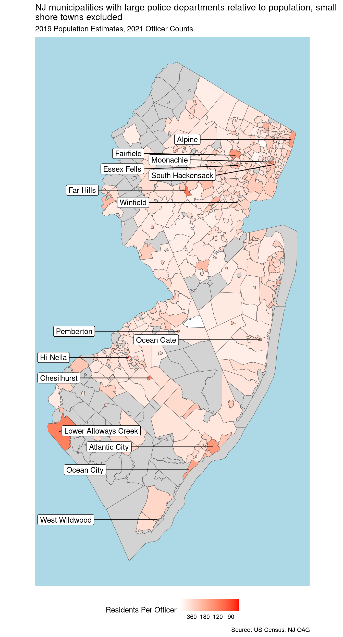
Hi-Nella is the new leader, followed by Far Hills and Lower Alloways Creek. It is not clear if either Far Hills or Lower Alloways Creek is including part-time officers, like Hi-Nella does. The size of the Lower Alloways Creek PD may be related to the presence of the nuclear power plant. West Wildwood and Ocean Gate should probably be considered part of the Jersey Shore, though they don’t actually border the ocean.
Geographically, no clear pattern appears, except perhaps that South Jersey is somewhat over-represented:
# Add the residents_per_officer to the map, excluding shore towns
map_with_values <-
  left_join(nj_municipality_map, officer_count_pop_core, by = "GEOID")

# Map the officer density
labels <- map_with_values %>%
  slice_min(n = 15, order_by = residents_per_officer) %>%
  arrange(desc(INTPTLAT))

# Plot the map
scale_breaks <- c(90, 120, 180, 360)
ggplot(map_with_values) +
  geom_sf(aes(fill = residents_per_officer, geometry = geometry, size = .2 )) +
  ggrepel::geom_label_repel(
    data = labels,
    mapping = aes(label = NAME, geometry = geometry),
    stat = "sf_coordinates",
    nudge_x = -.7,
    min.segment.length = 0
  ) +
  scale_size_identity() +
  scale_fill_gradient(
    na.value = "lightgrey",
    low = "white",
    high = "red",
    trans = "reciprocal",
    breaks = scale_breaks,
    name = "Residents Per Officer"
  ) +
  labs(
    title = str_wrap(
      "NJ municipalities with large police departments relative to population, small shore towns excluded"
    ),
    subtitle = "2019 Population Estimates, 2021 Officer Counts",
    caption = "Source: US Census, NJ OAG"
  ) +
  theme(
    axis.ticks = element_blank(),
    axis.text.x = element_blank(),
    axis.text.y = element_blank(),
    axis.title.x = element_blank(),
    axis.title.y = element_blank(),
    panel.background = element_rect(fill = "lightblue"),
    panel.grid.major = element_line(color = "lightblue"),
    legend.position = "bottom"
  )
Next
In subsequent posts, we dig in further, looking at:
- Municipality demographics (US Census)
- Department diversity (
njoagleodpackage) - Use of force (
njoaguofpackage)
The municipal PD officer counts are also available in the FBI Uniform Crime Reports.↩︎
Note that the tidycensus package needs to be supplied with a census API key, which is not shown in the code snippet. See here.↩︎
The FBI UCF claims that the numbers are for “Full-time Law Enforcement Employees”, and lists 13 as the size of the Hi-Nella PD in 2018. Since Hi-Nella is evidently improperly including part-time officers its report to the FBI, we suspect that the inclusion of part-time officers in the NJ OAG report is also an error, and that most municipalities in the NJ OAG Law Enforcement Officer Diversity data set are including only full-time officers. According to the NJ OAG, all officers in the dataset are full-time.↩︎